Heptabase Notes

Question: How to develop scheduling policy?

In previous chapters, we learned about Processes and how the operating system can choose whether to switch to executing other processes through the mechanism of a timer interrupt.

So, in this chapter, we will begin to discuss how the operating system decides which process to execute next.

In this chapter, all mentioned Jobs can be understood as a Process.

Simplifying the Problem #

To simplify the problem, we first make a few important assumptions and then gradually remove these assumptions to come closer to real-world situations.

1. Each job has the same execution time.
2. All jobs appear at the same time.
3. Once a job starts executing, it must run to completion.
4. All jobs only use the CPU and do not involve any other I/O operations.
5. We can know the execution time of all jobs.

Metrics #

Before we begin discussing how to design a Scheduler, we can first consider what criteria we should use to judge whether a design is good or not.

Turnaround Time #

Turnaround time refers to the time at which the job completes minus the time at which th job arrived in the system.

Response Time #

Response time refers to how long it takes for a job to start after it arrives.

Implementing Various Schedulers #

FIFO #

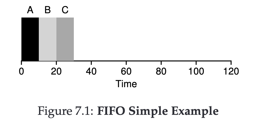
This is the simplest approach, executing jobs regardless of circumstances.

Turnaround time = (10+20+30) / 3

Once we remove the first assumption, FIFO encounters a problem.

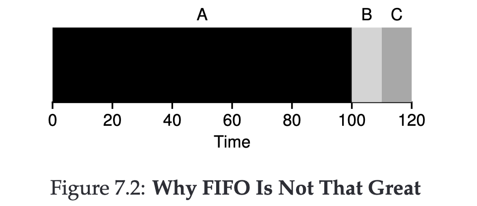
If the first job executed takes a long time, this will significantly increase our Turnaround time.

Turnaround time = (100+110+120) / 3

Shortest Job First (SJF) #

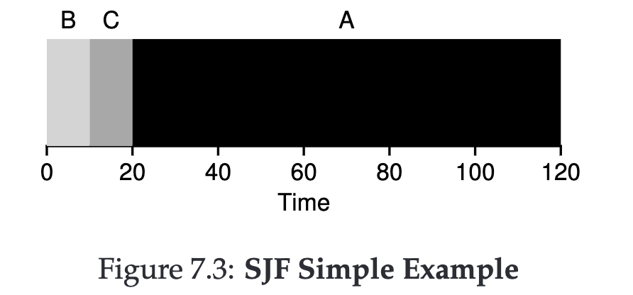
To solve the minor issue with FIFO, we can choose to execute shorter jobs first before the longer ones. (I know this isn’t realistic, but remember our assumptions?)

Turnaround time = (10+20+120) / 3

Let’s make things more interesting, if we remove the second assumption (jobs arrive simultaneously) on the basis of SJF.

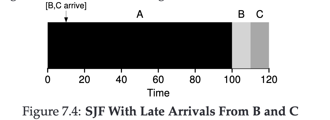
Because jobs don’t arrive simultaneously, and our third assumption is that once a job starts, it must run to completion.

Thus, our Turnaround time becomes = (100 + (110-10) + (120-10)) / 3

Shortest Time-to-Completion First (STCF) #

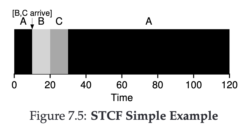
We can lift the third assumption (a job must run to completion once it starts), to address the problem faced by SJF and improve Turnaround time.

This means when a new job arrives, if its execution time is shorter than the remaining time of the currently executing job, we switch to the new job.

Turnaround time = ((120-0)+(20-10)+(30-10)) / 3

Round-Robin #

While the above methods effectively improve Turnaround time, they are not conducive to improving response time.

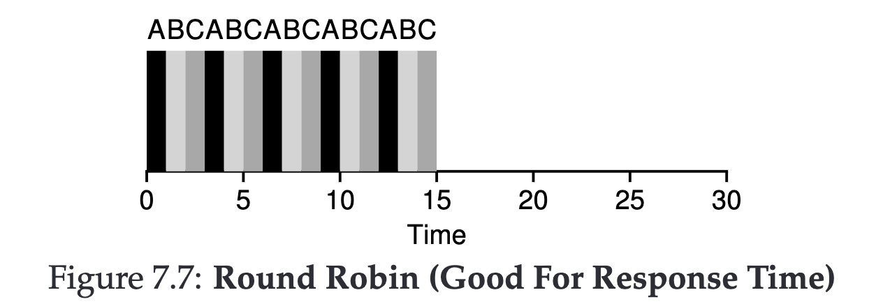
The concept of Round-Robin is simple; we can run each job for a set period, assume 1s (this period must be a multiple of the timer-interrupt).

If you want to improve your response time, you could adjust it so that it switches jobs every 500 ms.

But also remember, each switch has a cost (remember the context switch tasks the operating system has to do from previous chapters?)

For example, if you set it to switch jobs every 10ms, and the context-switch cost is 1ms, then about 10% of the time is wasted on context-switches.

I/O Operations #

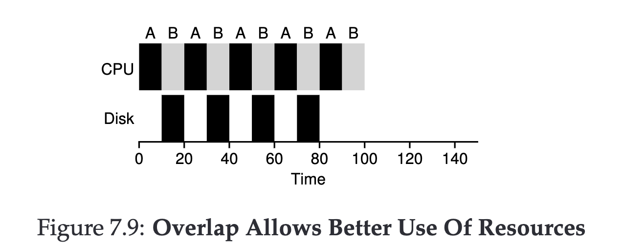
Jobs inevitably involve I/O operations, so we’ve lifted the fourth assumption. Because we’ve already lifted the third assumption, this task becomes much easier.

The operating system will pause the job waiting for I/O and switch to executing other jobs to improve CPU efficiency.

The Final Problem #

At this point, you’ll realize that one assumption hasn’t been lifted yet. All the above discussions are based on knowing the execution time of jobs, but in real life, we almost can’t achieve this.

We will discuss this issue in the next chapter.